Spectrophotometric Errors: |

For spectrophotometric errors, consider the following model instrument:


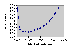
As %T approaches 100% and A approaches zero, the uncertainties in measuring %T dominate the error in A. It can be shown that the absolute error in A due to %T error = Error in %T*0.434/%T. [For example, in a Spectronic 20 the instrumental noise is 0.5%T. At an Absorbance of 0.100 (%T=79.4%) the error is 0.5%T*0.434/79.4%T=0.003 A, a 3% error in A.] In simpler terms, at low concentrations the instrument can no longer "see" the color present with any accuracy.
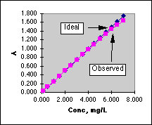
As %T approaches zero and A approaches infinity, we run out of light to measure when the concentrations become too high. In addition to the random errors inherent in measuring very low light levels, Stray Light limits our ability to measure highly absorbing solutions. All spectrophotometric instruments allow some of the light to bypass the cell and add to the light reaching the detector. In a Spectronic 20, this amounts to 0.5%T. So even if our sample is so concentrated that it absorbs nearly all the light that is put into it, the detector will not produce a readout of 0.0 %T. The actual %T is:

A spreadsheet analysis computes the actual errors:
Absorptivity
|
0.25
|
| Path
Length, b
|
1
|
| Po
|
100
|
| Stray
Light %
|
0.5
|
| Pstray
|
0.5
|
| Error
in %T
|
0.5
|
conc
|
Ideal
A
|
Ideal
%T
|
P
|
P+Pstray
|
%T
observed w Stray Light
|
A
observed w Stray Light
|
Combined %error in A
|
| 0.100
|
0.025
|
94.41
|
94.41
|
94.91
|
94.43
|
0.025
|
9.21
|
| 0.500
|
0.125
|
74.99
|
74.99
|
75.49
|
75.11
|
0.124
|
2.39
|
| 1.000
|
0.250
|
56.23
|
56.23
|
56.73
|
56.45
|
0.248
|
1.68
|
| 1.500
|
0.375
|
42.17
|
42.17
|
42.67
|
42.46
|
0.372
|
1.58
|
| 2.000
|
0.500
|
31.62
|
31.62
|
32.12
|
31.96
|
0.495
|
1.66
|
| 2.500
|
0.625
|
23.71
|
23.71
|
24.21
|
24.09
|
0.618
|
1.83
|
| 3.000
|
0.750
|
17.78
|
17.78
|
18.28
|
18.19
|
0.740
|
2.09
|
| 3.500
|
0.875
|
13.34
|
13.34
|
13.84
|
13.77
|
0.861
|
2.44
|
| 4.000
|
1.000
|
10.00
|
10.00
|
10.50
|
10.45
|
0.981
|
2.89
|
| 4.500
|
1.125
|
7.50
|
7.50
|
8.00
|
7.96
|
1.099
|
3.45
|
| 5.000
|
1.250
|
5.62
|
5.62
|
6.12
|
6.09
|
1.215
|
4.16
|
| 5.500
|
1.375
|
4.22
|
4.22
|
4.72
|
4.69
|
1.329
|
5.04
|
| 6.000
|
1.500
|
3.16
|
3.16
|
3.66
|
3.64
|
1.438
|
6.15
|
| 6.500
|
1.625
|
2.37
|
2.37
|
2.87
|
2.86
|
1.544
|
7.52
|
| 7.000
|
1.750
|
1.78
|
1.78
|
2.28
|
2.27
|
1.645
|
9.22
|


In the working curve at the left we see the departure from linearity above A=1.0. In the graph on the right we see that the "best" range in which to use a Spectronic 20 lies between A=0.1 and A=1.0, with a minimum around 0.4 Absorbance. Outside of this range the errors increase rapidly.
David L. Zellmer, Ph.D.This page was last updated on 29 March 1997
Department of Chemistry
California State University, Fresno
E-mail: david_zellmer@csufresno.edu