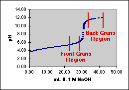
Gran's Plots for pH TitrationsIncludes Error Analysis for a Least Squares Fit
©David L. Zellmer, Ph.D. |

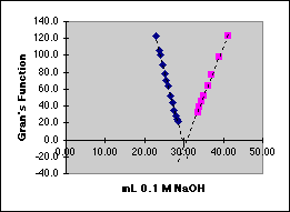
Frontside Grans = (Vo+Vml)*10^(pH1front - pH)
Backside Grans = Scale Factor*(Vo+Vml)*10^(pH-pH1back)
Remember that [H+] = 10-pH. and [OH-] =10-(14-pH). By setting the pH1front term to the initial Frontside pH value, we make our first Gran's value equal to (Vo+Vml) a value that our spreadsheet will easily plot. By making pH1back equal to the last pH value we can place both graphs on the same plot. The Scale Factor removes small differences between the two, mostly for cosmetic reasons. If you wish to compute the Scale Factor, it is simply (Vo+VmlFirst)/(Vo+VmlLast).
The designations "Front" and "Back" as used above work for a strong base as the titrant. You will need to make appropriate changes when titrating with an acid. [Hint: Hydrogen ion increases as we titrate with an acid.]
Our parameter table is:
A
|
B
| |
| 6
|
Vo
|
100
|
| 7
|
pH1
front
|
5.42
|
| 8
|
pH1
back
|
12.01
|
| 9
|
Scale
Factor
|
0.87
|
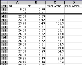
Our first Gran's Value found in cell C49 in the figure below would then be:
Cell C49 = ($B$6+A49)*10^($B$7-B49)
For the statistical analysis we will use some special features of the Excel spreadsheet that depend on the Define Name... capability.
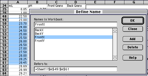
Rather than typing in $A$49:$A$61 every place we need our array of Frontside X-values, we will give this array the name FrontX. The array in column C will be given the name FrontY. To do this, drag the mouse over A49 to A61 to select it, then choose Insert/Name/Define... from the Insert Menu. (Versions of Excel other than 5.0 Mac may have Define Name... in other locations.) A dialog box will come up that will let you enter the name you want.


| m
|
SLOPE(FrontY,FrontX)
|
| sr
|
STEYX(FrontY,FrontX)
|
| M
|
number of values for an average y-value.
|
| N
|
number
of data points in the line = COUNT(FrontX)
|
| Sxx
|
(N-1)*STDEV(FrontX)^2
|
| y
bar sub c
|
the average instrument response used to compute an average y-value.
|
| y
bar
|
AVERAGE(FrontY)
|
But when our "average y-value" is the x-axis itself, y bar sub c becomes zero and the M term is removed, since y bar sub c is no longer an experimental value. The modified formula is then:


The slope, m, had previously been computed in cell $E$7.
To see how our "quick and dirty" method compared with the better calculation above, compare
Front
|
Back
| |
| Volume
intercept
|
29.50
mL
|
30.70
mL
|
| steyx/slope
(1-sigma)
|
0.15
|
0.065
|
| 2*steyx/slope
(2-sigma)
|
0.30
|
0.13
|
| s
sub c at y=0
|
0.091
|
0.056
|
| 95%CL
based on s sub c
|
0.20
|
0.14
|
The 2-sigma limits are very similar to the 95% CL, as is generally the case, so the simpler calculations based on a simple calculation of the standard deviation can be used. If you have the time and the computing power, using the full equations is still better and is more defensible in a formal report.
For the real data used in this example, our choice of Gran's regions has resulted in two volume intercepts which are significantly different from each other.
David L. Zellmer, Ph.D.This page was last updated on 5 April 1997
Department of Chemistry
California State University, Fresno
E-mail: david_zellmer@csufresno.edu