A Basic Working Curve Plot with Linear Least Squares Calculation of Concentration

©David L. Zellmer, Ph.D.
Department of Chemistry
California State University, Fresno

A brief tutorial on basic graphing and using the LINEST() function in Microsoft Excel follows the figure below. Those viewing this page using a browser without Frames will need to scroll up and down to match the red numbers in the figure with the explanations in the text.

Put in labels for all your data so you can remember what all the numbers are.
Enter your data for concentration and absorbance (or other X,Y data) in two columns as shown in columns A and B. For the unknown, all we have is its absorbance, so "unk" is put in the concentration column. All the other numbers shown will be calculated later.
Before attempting any least squares analysis, we first must PLOT our data to determine if it looks like a straight line.
Select your data to plot by selecting it with the mouse. Here we have selected from A7 to B10. All versions of Excel will do a true X-Y scatterplot, but other spreadsheets may not--Microsoft Works, version 3.0 or earlier, for example, cannot be used for this.
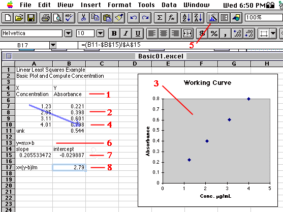
Now select the Chart Wizard , available in most recent versions of Excel (3, 4 and 5). A simpler version of the Wizard gives you only one choice--X-values in first column for a scatterplot--but won't do the labeling for you. A cross-hair will appear. Use the mouse to drag a charting area as shown in the graphic. Once the area is drawn and the mouse released, the Wizard will prompt you with the information needed to make the graph. Here we have chosen an X-Y(ScatterPlot) with datapoints shown, but no connecting lines or grids. One of the dialog boxes will permit you to enter the chart title, and titles for the X and Y axes. At the completion of the Wizard questions, the chart shown will appear.
The data appear to be linear, so we will compute the slope (m) and intercept (b) for the equation for a straight line y=mx+b. To do this we will use an Excel function called LINEST(y-array, x-array).
LINEST will generate TWO values, so we must enter it into two cells, using a special command when entering it.
- Label two cells slope and intercept as shown in A14 and B14. The computer doesn't need these labels, but you will.
- Use the mouse to select the two cells (A15 to B15) underneath them. With the cells selected type in =LINEST(B7:B10,A7:A10). DON'T HIT THE ENTER KEY YET!
- To enter this special formula, hold down the Command Key while pressing Enter (Mac), or Control-Shift-Enter (on a PC). The slope and intercept will appear in the two selected cells.
If we solve y=mx+b for x, we get x=(y-b)/m. This formula has been typed in as a label for the benefit of the humans who will be reading this spreadsheet. The computer could care less. In cell B17 we type the spreadsheet formula =(B11-$B$15)/$A$15. Enter this in the usual way (press Enter or Return) to calulate the X-value (concentration) that goes with the Unknown Y-value (absorbance) that you put into cell B11 earlier.
Congratulations. You have just used Linear Least Squares analysis to compute the concentration of your unknown. To draw the least squares line on the graph, or to estimate errors, see the more advanced LLS methods provided on this Web site.

Return to LLS Basic Master Page

For questions or comments, contact Dr. David Zellmer at david_zellmer@csufresno.edu.

Last Updated: 8 February 1997