A First Order Fit to the data used to construct a working curve follows the equation:

Failure to check our data for linearity before performing our usual Linear Least Squares (LLS) analysis will generate a large error if the data are curved rather than straight.

In the example above we see a standard LLS first order fit. How do we know that this is a poor choice? Do the data really have the amount of scatter shown? Shouldn't we just accept the value of 9.19 +or- 1.07 µg/mL? These questions do not have obvious answers. There is no reliable formula or computer analysis that can tell the difference between scattered data and curved data when the number of data points is small. Instead, we must rely on what a professional chemist would expect to see.

1) We expect the error for this method to be around 1 or 2%. Our results show (1.07/9.19)*100 = 12%.

2) We have been warned that at moderately high absorbance values we might get non-linearity when doing atomic absorption.

3) Consulting the manual for our atomic absorption spectrometer, we find that it has built-in software for a "three-point calibration." Three points are the minimum needed to do a curved, second-order fit. This tells us that doing a second order fit on these data should be professionally acceptable.

We will follow the equation:

Graph the data using a Scatter (XY) plot in the usual way. Then click on the data to select it. From the menu choose Chart/Add Trendline.... From the window that appears, select Polynomial of Order 2.

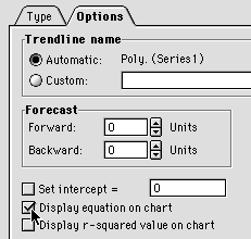
Under Options, choose Display Equation on Chart

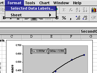
The equation we get on the chart needs to be fixed up a bit before we can use it. (1) It is too small to see properly, and (2) the coefficients don't have enough significant figures for accurate use. Click on the equation on the chart to select it, then choose Format/Selected Data Labels...

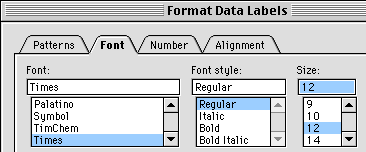
From the window that appears, make the Font size 10 or 12 so you can see it, then click the Number tab and set Scientific Notation with three places after the decimal.

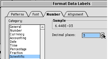
You can now see the equation and have enough significant figures so you can use the coefficients.

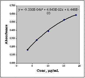
Another little trick you can use to see the coefficients properly is to select the equation on the graph, drag your mouse over the equation to select it as text, then Copy it, and Paste it into a convenient cell where you can easily copy and paste individual coefficients. You could do this directly from the graph, of course, but selecting things from graphs can be tricky at times.

You can now plug your Y-value of 0.347 Absorbance into this equation and solve the resulting quadratic equation for X to get the concentration. Another way would be to make the graph much larger, put in gridlines, and read the value from the graph.

You can let Excel solve the quadratic equation for you using Goal Seek.

First, make a copy of the original data and paste them into the spreadsheet starting at row 24. Then in column C rewrite the polynomial equation, substituting references to the values in column A for the X values.

Cell C27= -0.000933*A27^2 + 0.04843*A27 + 0.006448

Cell D27=B27-C27

The difference between our real data and that calculated from the second order polynomial is found in column D. We can use these values to estimate our error. It looks like we have an error of about (0.006/0.4)*100 = 1.5% near the center of this working curve. That seems about right.

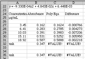
We are now read to use Goal Seek to solve our equation. Copy row 32 and Paste it into 35 so you can play with it. Look at the graph and make a guess at what the concentration should be for an absorbance of 0.347. It looks like the value should be around 9 µg/mL. Put that value into A35. Values now appear in C35 and D35.

Now click on the Difference in Cell D35 and select Tools/Goal Seek...

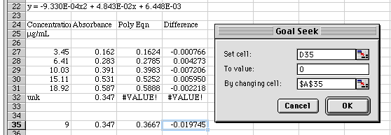
Tell Goal Seek that we want to set the Difference to 0 by changing the concentration value in A35. Click OK.

Goal Seek hunts for a value of concentration until the difference is less than 0.001. This works well for these numbers. We find that we have a concentration of 8.38 µg/mL for our unknown. Our estimated error for this will be 1.5% of 8.38 or about 0.13.

Final reported value: 8.38 +or- 0.13 µg/mL. Compare this to the value of 9.19 +or- 1.07 µg/mL we would have gotten had we stayed with good old linear least squares analysis. The second order fit works much better.