Standard Addition

Standard Addition

Standard addition must be used whenever the matrix of a sample changes the analytical sensitivity of the method. In other words, the slope of the working curve for standards made with distilled water is different from the same working curve made up in swamp water (or whatever your real world matrix happens to be).

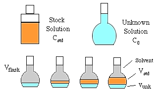
To do constant volume standard addition we need the following solutions and glassware.

A constant volume (Vunk) of the unknown solution is added to each of four volumetric flasks of volume Vflask. Then a series of increasing volumes of stock solution are added (Vstd). Finally, each flask is made up to the mark with solvent and mixed well. The concentration and volume of the stock solution added should be chosen to increase the concentration of the unknown by about 30% in each succeeding flask.

The actual concentration of the analyte in any given flask will be given by:

The instrumental response to the analyte will be R = (K)(concentration), so

Now set Csa = CstdVstd/Vflask.

After measuring the response for a series of standard additions, we plot the results, then extrapolate to y = 0 to get the value of that Csa would need to be to equal the response of the unknown. We use this negative value to compute Co.

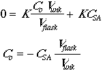
Here is an example of this calculation carried out on a spreadsheet using simulated data. Remember that the Parameters section sets up the simulation, while the Calculations section carries out the analysis in much the same way you would do it.

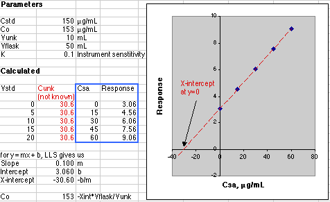
The data in the blue box are plotted in the graph. The figures shown in red in the Calculated section would not be known to the analyst. All the analyst knows is the concentration due to the additions of the standard, so please don't try to create the figures in red when working up your own data! The point here is that the instrument is responding to the sum of the unknown and standard addition analyte.

A simple Linear Least Squares (LLS) analysis is made using the SLOPE(y-array, x-array) and INTERCEPT(y-array, x-array) functions of Microsoft Excel. From y=mx+b we calculate the value of x at y=0, which is -30.60, Co = -(-30.60)*50mL/10mL or 153 µg/mL. This agrees with the value of Co of 153 µg/mL set in the Parameters section of the simulation.

A more advanced simulation adds the effect of instrumental uncertainty. The analyst must calculate both the value of Co and its associated error. See Gran's Plotting for pH Titrations for full details on computing the error of an X-axis intercept using Excel. A quick example will be given here.

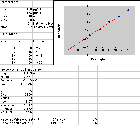
Our instrumental error was set at 0.2 out of a maximum response of about 10, or a 2% error. The effect of this error on the final result is quite a bit larger than 2%. The 95% Confidence Limit of Co is 32.6 for a value of 139.3, or a 23% error! Some analysts prefer to use the "1-sigma" error, which is much smaller. Here that would be "s sub c, y=0" or a 2.047 error in the Csa value of 27.85 or 7.4% error.

With the errors this large, the analyst would have to report the result as 140 +or- 30 µg/mL. The extra significant figures would not be justified.

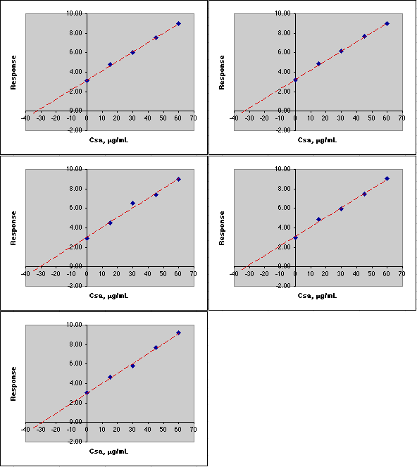
If you think these computed errors seem excessively large, consider the animation below where the simulated analysis is repeated over and over. Note how the X-intercept bounces around.

For questions or comments, please contact:

Dr. David L. Zellmer
Department of Chemistry
California State University, Fresno
david_zellmer@csufresno.edu